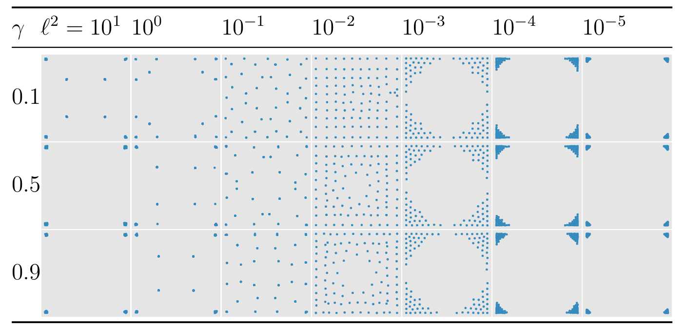
The idea is to prove convergence of the ABC posterior to the true posterior as \(\epsilon \to 0\). I’ll cover previous proofs, extend them, and relate them to the key underlying mathematical results.

Bayesian setting

Consider the Bayesian setting with:

• Prior density \(p(\theta)\)
• Model density \(f(y \vert \theta)\)
• Observations \(y_0\)

I’ll assume \(\theta \in \mathbb{R}^d\), \(y \in \mathbb{R}^n\), and that \(p(\cdot)\) and \(f(\cdot | \theta)\) are densities with respect to Lebesgue measure. Therefore \(f(\cdot | \theta)\) is an integrable function.

Now let:

Throughout, all integrals are over the full \(\theta\) or \(y\) space, unless the domain of integration is specified.

I’ll assume:

• A1: \(Z>0\) (the observations are supported under the prior and model)

Later I’ll also use the notation:

noting that \(Z(y_0) = Z\) and \(\int Z(y) dy = 1\).

Remarks:

• I think all the results below also hold for discrete \(\theta\) and \(y\) distributions. I think it’s also fine for \(p(\cdot)\) to be a density with respect to a more general measure but I’m not whether this is the case for \(f(\cdot|\theta)\). There are some comments below on where the proof needs modification for these cases.
• Edit May 2023: A case not covered by this proof is when \(y\) is continuous but \(y | \theta\) is singular with respect to Lebesgue measure. This can occur if a component of \(y\) is a deterministic function of \(\theta\), and can produce a posterior which is singular with respect to the prior, thus requiring more sophisticated measure theoretic tools.

ABC posterior and likelihood

Many ABC algorithms produce samples from the ABC posterior \(p_\epsilon(\theta | y)\). For an overview see for example Sisson et al (2018). The ABC posterior can be defined as follows:

Here \(K_\epsilon\) is a kernel function and \(\epsilon > 0\) is a bandwidth. We’ll consider kernels of the form: \(K_\epsilon(y) = \epsilon^{-n} K(y/\epsilon),\) where \(K\) is base kernel, a non-negative function \(\mathbb{R}^n \to \mathbb{R}\). We assume:

• K1: \(K\) is bounded
• K2: \(\int K(y) dy = 1\).
• K3: \(K(y) > 0\) for \(\vert \vert y \vert \vert \leq 1\) (where \(\vert \vert \cdot \vert \vert\) is the Euclidean norm).

The most common base kernel used in ABC is the uniform kernel:

were \(1[\cdot]\) is an indicator function and \(k_U\) is a suitable normalising constant (volume of an \(n\)-ball). Also common is the Gaussian kernel:

where \(k_G = (2 \pi)^{n/2}\).

Remarks:

• The ABC likelihood and posterior are similar to kernel density estimates, which is where the bandwidth terminology is taken from.
• The \(k_U\) and \(k_G\) constants ensure that K2 is satisfied. In a lot of ABC literature this plays no role, so the kernels are often defined without these constants.
• Under K2, \(K\) and \(K_\epsilon\) are probability density functions. The ABC posterior is then the posterior under the model plus independent noise from \(K_\epsilon\) (see Wilkinson 2013).
• In other contexts, the Gaussian kernel is known as the heat kernel.

ABC posterior convergence

The goal is to show that the ABC posterior converges in distribution to the posterior in the limit \(\epsilon \to 0\).

Previous work

Rubio and Johansen (2013) (Proposition 1) prove ABC posterior convergence given:

• A kernel (defined slightly differently to above) with bounded support.
• Some continuity and local boundedness requirements on \(f(y \vert \theta)\).

Prangle (2017) (Theorem 1, in the supplement) proves ABC posterior convergence for almost all \(y_0\) given:

• A uniform kernel.
• A general choice of \(f(y \vert \theta)\).

The latter proof is based on the Lebesgue differentiation theorem (LDT), discussed below.

The aim of this post is to generalise the result to a general likelihood and kernel satisfying K1-K3.

The two papers above are of most relevance to this post, but other related work on ABC convergence results includes the following:

• Blum (2010), Fearnhead and Prangle (2012) and Biau (2015) derive results on the accuracy of estimates from ABC algorithms. These involve dealing with the error in the ABC posterior, as well as other sources of error.

• Barber et al (2015) prove the convergence of ABC posterior expectations for a uniform kernel.

• Bernton et al (2019) (Proposition 3.1) prove ABC posterior convergence following the approach of Rubio and Johansen, but under different conditions relevant to their purposes. Amongst other authors, they also consider a different asymptotic regime: \(n \to \infty\) (large number of observations).

Approximations of the identity

The key tool in the proof is the following result. I’m using the definitions and statement from Stein and Shakarchi “Real analysis: measure theory, integration, and Hilbert spaces” (2005).

For an integrable function \(g:\mathbb{R}^n \to \mathbb{R}\) (such as any probability density function), consider a convolution:

Stein and Shakarchi, Theorem 2.1 of Chapter 3, states that

for almost all \(y_0\) if \(K_\epsilon\) is an approximation of the identity (AOTI). Conditions K1-K3 are sufficient for \(K_\epsilon\) to be a AOTI.

Remarks:

• For small \(\epsilon\), the convolution operation approximates the identity operation. This is what the AOTI name refers to.
• I use AOTI to refer to both the theorem, and the class of kernels for which it holds. Hopefully the distinction is clear from the context.
• The LDT can be viewed as the special case of AOTI when \(K\) is the uniform kernel. Typically the LDT is proved first, and used to derive AOTI.
• The analogous result to AOTI for discrete \(y\) is trivial. Therefore the main ABC convergence proof holds for discrete \(y\) with little modification. However I’m not sure what conditions are needed if \(f(\cdot|\theta)\) is a density with respect to a more general measure.
• AOTI kernels are possible which do not take the form \(K_\epsilon(y) = \epsilon^{-n} K(y/\epsilon)\). One application of this is to adaptive ABC distance functions (as in Prangle 2017).
• The full theorem statement in Stein and Shakarchi has more details on the definition of an AOTI kernel, and which \(y_0\) points the theorem holds for (the Lebesgue points of \(g\)).
• Edit June 2023: In the context of AOTI, \(K_\epsilon\) is sometimes known as a mollifier.

ABC convergence proof part 1: pointwise convergence of the ABC likelihood

Applying AOTI gives that for almost all \(y_0\):

Remark: Rubio and Johansen give an elementary proof of this result for all \(y_0\) in the case of continuous \(f(\cdot \vert \theta)\), and some restrictions on \(K_\epsilon\). AOTI is needed for non-continuous \(f\).

ABC convergence proof part 2: convergence of the ABC normalising constant

We have:

So applying AOTI gives \(\lim_{\epsilon \to 0} Z_\epsilon = Z(y_0) = Z\) for almost all \(y_0\).

Remarks:

• Rubio and Johansen give a proof using the dominated convergence theorem, which requires boundedness conditions on \(f\).
• This proof holds when \(p(\theta)\) is a density with respect to counting or more general measure.

ABC convergence proof part 3: conclusion

It remains to observe that for almost all \(y_0\):

Note that A1 is implicitly used above. Finally, convergence in distribution follows from Scheffé’s theorem.

This is the second part of a blog post on a preprint by Sophie Harbisher, Colin Gillespie and me. The first part was about the computational benefits of using the “Fisher information gain” (trace of the Fisher information matrix) as a utility function in Bayesian experimental design. This part is on theoretical justification for its use.

I’m going to start with a quick intuitive explanation, by analogy with the popular Shannon information gain utility. Then I’ll go over a more detailed argument based on decision theory.

Shannon information gain

One way to summarise the information provided by data \(y\) on parameters \(\theta\) in a Bayesian analysis is through the Kullback-Leibler divergence from the prior to the posterior:

(Recall that \(\tau\) represents the experimental design.)

The quantity inside the expectation is known as the Shannon information gain (SIG):

Maximising the expected SIG or expected KL divergence gives the same optimal design. (Recall that the expectation is over \(\theta, y\) from the prior and model, given \(\tau\).)

However evaluating or estimating (2) is hard, because it requires estimating the posterior density. Even if posterior samples are available from Markov chain Monte Carlo then getting a density estimate is still non-trivial.

An alternative form of the SIG can be found by applying Bayes theorem:

where \(p(y; \tau) = \int p(\theta) f(y \mid \theta; \tau) d\theta\) is the evidence (aka marginal likelihood or normalising constant).

Substituting this into (2) gives

The difficulty now is estimating the log-evidence. This is easier than estimating a posterior density but still computationally demanding.

Fisher information gain

The approach above compares posterior and prior log densities by looking at their difference. This is challenging because it requires correctly normalising the posterior density by computing the evidence. An alternative is to look at the gradient of the difference. As we shall see, this avoids the need to calculate the evidence.

One way to modify the KL divergence to use a gradient gives

where

• \(\|x\| = \sqrt{x^T x}\) is the Euclidean norm
• \(\nabla\) represent gradient with respect to \(\theta\)

Stephen Walker refers to this as the Fisher information distance, and it is easy to check this is a well defined divergence from prior to posterior.

The quantity inside the expectation in (3) is

Earlier we used Bayes theorm to show that

Taking the gradient gives

Note that the evidence term vanishes as it doesn’t depend on \(\theta\) and so has zero gradient.

Substituting this into (4) gives

and taking the expectation over \(y\) gives

which turns out to equal the trace of the Fisher information. We call this the Fisher information gain due to the similarity to the Shannon information gain.

Summary so far

We started by considering the KL divergence, based on the difference in prior and posterior log densities, and showed this derived the standard SIG utility function. We then considered an alternative divergence based on the gradient of the difference in prior and posterior log densities, and derived our FIG utility function. The benefit of taking the gradient is that it removes the hard-to-calculate evidence term from the utility. This allows easier optimisation of the expected FIG than the expected SIG.

The arguments so far are closely related to those in Stephen Walker’s paper. Also the idea of looking at log density gradients to avoid normalising the posterior may seem familiar from Hyvärinen’s score matching work. We’ll see below that there is a mathematical connection.

One other thing to note is about pseudo-Bayesian utilities. Ryan et al defined a experimental design utility to be fully Bayesian if it’s a function of the posterior and pseudo-Bayesian if not. On the face of it \(\mathcal{U}_{\text{FIG}}\) appeared to be pseudo-Bayesian. However we can now see that it is in fact the expectation of \(\mathcal{U}_{\text{diff}}\), which is fully Bayesian. Therefore \(\mathcal{U}_{\text{FIG}}\) gives the same optimal design as a fully Bayesian utility. This suggests working with a more foundational idea of what is a justifiable utility for Bayesian experimental design.

Bayesian decision theory and experimental design

A foundational approach to Bayesian statistics is through decision theory. This was applied to experimental design by Dennis Lindley amongst others. In particular, Jose Bernardo provided a decision theoretic derivation of the SIG utility. Our work shows that a similar argument can produce the FIG utility.

Experimental design can be viewed as the following decision problem.

1. The experimenter selects a design, \(\tau\).
2. Nature selects some parameters, \(\theta\) (unseen by the experimenter).
3. Nature generates some data \(y\) based on \(\tau\) and \(\theta\).
4. The experimenter selects an action based on \(y\).
5. The experimenter receives a base utility \(\mathcal{V}\) depending on \(\tau, \theta, y, a\).

(We use the term “base utility” given a particular action to distinguish with “utility” \(\mathcal{U}\) which was discussed in part I and will be introduced again shortly!)

As in part 1 we assume that \(\theta\) and \(y\) come from a prior and model. The action could be a concrete decision - e.g. give a patient a particular treatment, pick government policy X over policy Y - in which case the base utility should ideally quantify the costs and benefits. We’re concerned with coming up with a generic approach when these details aren’t available.

We’ll consider the action to be making a summary of knowledge about the parameters given the data. The action could be a point estimate for \(\theta\), which allows a base utility such as mean squared error. Instead we follow Bernardo who suggested instead letting the action be a distribution for \(\theta\). Suitable base utilities are then supplied by the theory of proper scoring rules, discussed below.

At step 4 the experimenter wants to pick the action maximising the expected value of \(\mathcal{V}\) given \(\tau\) and \(y\). We can define a utility function \(\mathcal{U}(\tau, y)\) which equals the maximum expected \(\mathcal{V}\). We can then use the framework of part I and pick the design which maximises the expected \(\mathcal{U}\).

Scoring rules

A scoring rule \(S(q,\theta)\) measures the quality of a prediction, here in the form of a density \(q\), given a realised value \(\theta\), by outputting a numerical value. Low scores represent good matches. Averaged over repeated predictions, the scoring rule can measure the quality of a forecaster e.g. of weather.

In our experimental design framework we can take \(\mathcal{V} = -S(a,\theta)\) i.e. base utility equals the negative of some scoring rule.

There are many scoring rules, e.g. see wikipedia, but these can be narrowed down by requiring a few properties

• A proper scoring rule has the following property. The expected score \(E_{\theta \sim p}[S(q,\theta)]\) is minimised by \(q = p\). For strictly proper scoring rule, this is the unique global maximum. The idea is that the optimal choice of \(q\) (i.e. minimising expected score) is its true distribution \(p\). Proper scoring rules encourage forecasters to report their true beliefs.

• A local scoring rule \(S(q,\theta)\) is one that depends only on \(q(\theta)\). So the score is only based on how likely \(\theta\) was predicted to be, not on predictions for events that did not occur.

The logarithmic scoring rule \(S(q,\theta) = -\log q(\theta)\) is the unique strictly proper local scoring rule (except that affine transformations are also allowed).

Other rules are possible if locality is relaxed slightly to allow \(S(q,\theta)\) to depend on derivatives of \(q(\theta)\). Allowing \(k\)th derivatives is called locality of order \(k\). An order-2 strictly proper scoring rule is the Hyvärinen score. (I’ll omit its formula as the details aren’t needed here.)

The logarithmic and Hyvärinen score seem good candidates to use to create a base utility.

Divergences from scoring rules

Given a scoring rule, various related quantities can be derived. One is a divergence

This is the excess expected score (remember high scores are bad!) from reporting \(q(\theta)\) rather than \(p(\theta)\) when the true density is \(p(\theta)\). It turns out that logarithmic score produces the Kullback-Leibler divergence (1), and the Hyvärinen score produces the Fisher information distance (3).

Experimental design based on scoring rules

Suppose we take \(\mathcal{V} = -S(a,\theta)\) in our experimental design framework. Then in step 4 of the framework the experimenter must choose a predicted density to minimise the expected score in step 5. If \(S\) is strictly proper, then the best choice is the true distribution of \(\theta\) given the available observations \(y\). This is the posterior \(p(\theta | y; \tau)\).

So in step 3 the experimenter will receive a utility of the negative expected score from the posterior. We can add a constant to the utility without affecting the decision procedure. Adding the right constant (\(E_{\theta \sim p(\theta | y; \tau)}[p(\theta)]\)) gives a utility of

where \(\mathcal{D}\) is the divergence derived from \(S\).

This argument shows that there is a decision theoretic justification for using a divergence derived from a scoring rule as a utility function in Bayesian experimental design. Using this argument, Bernardo showed that logarithmic score results in the KL divergence and SIG utility. In our paper we show that Hyvärinen score results in the Fisher information distance divergence and FIG utility.

Future research directions

We’ve shown a decision theoretic derivation of the FIG utility function in Bayesian experimental design.

But lots of questions remain for future work. First, what is the practical difference in the kind of designs that FIG produces compared to SIG (and other utility functions)? As discussed in part I, one of our examples produced a design with lots of replicated observation times/locations. Is FIG particularly liable to this? In our paper we speculate that maybe FIG is too risk seeking - too favourable towards designs that will occasionally produce extremely informative data.

Another question is what other utilities can be derived through decision theory? Perhaps we might be able to pick utilities with some desirable properties. Ehm and Gneiting and Parry, Dawid and Lauritzen recently investigated the class of proper local scoring rules, and it would be interesting to see what utility functions can result from them. Also a proper scoring rule \(S(q,\theta)\) could be modified to \(c(\tau,y) S(q,\theta) + d(\tau,y)\) and still be proper. Some choices of \(c\) and \(d\) might provide interesting alternative utilities. Finally perhaps we could reparameterise \(\theta\) before applying a scoring rule in an interesting way (similarly to the weighting scheme in part I).

Myself, my Newcastle colleague Colin Gillespie and our PhD student Sophie Harbisher recently uploaded a second version of a paper to arxiv. I thought this would be a good opportunity to blog about it while it’s fresh in my mind. The paper is on Bayesian experimental design, and how to scale it up to higher dimensional problems at a reasonable cost. In this first blog post I’m going to describe our method. Then in a second part I’ll explain some of the theory behind it.

You can also have a look at our code for this project on github.

Design of experiments

Before collecting some data we can often make some choices about how to do so. This can affect how informative the results are, and how expensive the collection process is.

The classic setting, from which the statistical terminology is taken, is where a design is selected before performing an experiment. Applications include:

• How many patients to use in a clinical trial.
• When to take measurements in a physics/biology experiment.
• Where to performing sampling in statistical ecology.

Similar settings also appear whenever a decision must be made about how to collect data for making a future task e.g.

• Where to place sensors in an autonomous vehicle.
• Where to evaluate a function for numerical integration.
• What parameter settings to use for runs of expensive climate simulators.

So classical design of experiments has a strong overlap with modern tasks in machine learning (e.g. active and reinforcement learning), probabilistic numerics and uncertainty quantification.

Design of experiments (DoE) has a long history in statistical research. The classic approach dates back to at least R A Fisher’s work in the 1920s-30s. In modern applications, it’s increasingly feasible to collect large amounts of data, so there’s an increasing emphasis on being able to select high dimensional designs.

Technical setup

We focus on the continuous version of DoE. That is, we wish to select a design made up of a fixed number of continuous quantities. For example we could be selecting measurment times, measurement locations, dose sizes etc. Mathematically we wish to select a \(d\) dimension vector \(\tau \in \mathbb{R}^d\).

We look at Bayesian experimental design, which uses the following decision-theoretic framework.

1. The experimenter must select a design, \(\tau\).
2. Nature selects some parameters, \(\theta\). We assume these are generated from a prior distribution \(\pi(\theta)\). (The parameters are unseen by the experimenter.)
3. Nature generates some data \(y\) based on \(\tau\) and \(\theta\). We assume this is generated from a model with likelihood function \(f( y \mid \theta; \tau)\). (These are seen by the experimenter.)
4. The experimenter receives a utility, \(\mathcal{U}\) depending on \(\tau, \theta, y\) (or a subset of these).

To use this framework we have to make assumptions about how nature produces data i.e. select a model and its likelihood function. The model typically depends on some unknown parameters \(\theta\). In a Bayesian approach we have to make assumptions their distribution i.e. select a prior. (Classic non-Bayesian DoE approaches face a similar issue, as they require picking a single nominal parameter value at which to assess the design.)

In Bayesian DoE, the optimal design is that maximising the expected utility (with respect to parameters and data). The computational challenge is to solve this optimisation problem - or come up with a close approximation - in a reasonable time.

Utility functions

The utility function \(\mathcal{U}\) is an important choice in DoE. It describes how useful the outcome is to the experimenter, taking into account both costs and benefits. Ideally a utility function could be designed for the particular application at hand. But this is often not possible and a generic utility function is used instead. This aims to measure how informative the experimental results are.

Most generic utility functions for Bayesian DoE involve the posterior density \(\pi(\theta|y;\tau)\) i.e. the distribution of the parameters given the design and data. The posterior summarises the experimenter’s knowledge of the parameters at the end of the experiment. The utility can be taken to be some scalar summary of the posterior - or the posterior compared to the prior - which describes how much information has been gained. Chaloner and Verdinelli, 1995 and Ryan et al, 2016 review many possible choices.

Computational challenges and existing methods

Calculating the posterior is typically computationally expensive. This makes Bayesian DoE challenging: we want to optimise expected utility but:

1. We can only evaluate a single utility at a time, not its expected value.
2. Even a single utility evaluation is expensive!

Many methods have been proposed for Bayesian DoE, including:

• Optimisation using MCMC, using Peter Müller’s algorithm.
• Coordinate ascent using Gaussian process optimisation, using the ACE algorithm of Overall and Woods.
• Approximating the expected utility by variational inference, using recent work of Foster et al.

However these all involve computational expense and/or approximations.

The FIG utility

We propose using a particular utility function which can be evaluated without posterior calculations. This makes the optimisation problem much simpler and cheaper, as we’ll see shortly.

We use what we call the Fisher information gain utility, \(\mathcal{U}_{\text{FIG}}(\theta, \tau)\). This is the trace of the Fisher information matrix. (As used in the non-Bayesian T-optimality criterion.) The Fisher information matrix is often available in closed form. Even if not, an unbiased Monte Carlo estimate can be formed in many applications (see Appendix E of our paper). In both cases it’s not necessary to infer the posterior.

Utility functions which avoid in the posterior in this way have been criticsed as being pseudo-Bayesian for not using the full information available from the data. However Stephen Walker recently showed that it turns out this utility produces the same optimal designs as a fully Bayesian utility (i.e. one which is a posterior summary). Our paper extends this argument by giving a foundational Bayesian derivation of the FIG utility through decision theory. The details are in the second part of this blog post.

Optimisation

We wish to maximise our expected utility,

We usually can’t evaluate this expectation. However we can compute an unbiased Monte Carlo estimate of its gradient,

where

• The \(\theta^{(k)}\)s are samples from the prior.
• \(\nabla_\tau\) represents gradient with respect to \(\tau\).
• \(\text{tr}\) represents trace.
• \(\mathcal{I}\) is the Fisher information matrix.

(Some regularity conditions are needed to allow swapping the order of expectation and gradient. Also the above is for the case where the trace of the Fisher information is easily differentiable e.g. using automatic differentiation. See our paper for more details.)

We can now use a powerful off-the-shelf method - stochastic gradient optimisation. We produce a sequence of \(\tau_i\) values where \(\tau_{i+1}\) equals \(\tau_i\) plus a step in the direction of \(\widehat{\nabla_\tau \mathcal{J}(\tau_i)}\). These converge to a local maximum of \(\mathcal{J}(\tau)\).

Lots of powerful adaptive stochastic gradient optimisation methods have recently been developed in the machine learning literature. They are typically used for learning the parameters of neural networks, and so can handle upwards of millions of unknowns. So we simply use the popular Adam algorithm for optimisation.

To summarise, we are in the nice position of simply applying standard gradient based optimisation to an easily available gradient estimator of our objective function \(\mathcal{J}\). In contrast, under most other utility functions, evaluating the objective function or its gradient is much more computationally demanding, and can necessitate using specialised optimisation algorithms or introducing approximations.

Example: geostatistical regression

Our paper contains an application to geostatistical regression. We are collecting spatial data assumed to follow a Gaussian process model with linear trends which we wish to learn about. Our method can find optimal designs of 100 locations in under a minute. The following figure shows some of the designs under various GP parameter choices. (See the paper for more details.) These show an interesting mix of regularly spaced points or concentration near the corners.

Difficulty 1: reparameterisation and weighting

One difficulty of our approach is that the Fisher information matrix is not invariant to reparameterisation, and therefore neither is our utility function. That is, simply by working with our parameters on different scales, we can end up with different designs. This is not a desirable property!

To deal with this we work with a weighted utility function. Our original utility function is the sum of the diagonal elements of the Fisher informatoon matrix. The weighted version instead uses a weighted sum of these elements. We propose an algorithm to adaptively select the weights so that we learn a similar amount of information on each parameter.

Difficulty 2: repeated design points, local maxima and post-processing

Another difficult of our approach is that it converges to local maxima of the expected utility rather than the desired global maximum. We found this particularly problematic in one example - see Section 6 of the paper. Here the designs represented a vector of times at which to make observations. Our optimal designs turned out to select repeated observations at two particular time points. Over multiple runs of our optimiser, there was considerable variation of how many design points were placed at each of these two times i.e. these outcomes formed many local maxima.

To deal with this we recommend post-processing our output if there are repeated points. We use the “ACE phase II” post-processing method implemented in the R package for ACE. This performs combinatorial optimisation by moving design points between replicated groups.

Whether or not there are repeated design points, we always recommend running our method multiple times from multiple starting designs. This checks for multiple local maxima.

It’s unclear whether repeated design points should be regarded as problematic or not. For example Binois et al recently argued that replicated observation times can be highly informative. Alternatively the tendency for replication in this example could represent some undesirable features of the utility function. I’ll discuss this further in the second part of this blog post.

Future research directions

We’ve used off-the-shelf stochastic gradient optimisation methods to allow fast Bayesian optimal design which can scale up to higher dimensional designs than most existing methods. These optimisers are typically designed for neural network applications. It would be interesting to see if variants can be designed specifically for experimental design. For example these could try to escape local maxima using tempering or line search.

Also all our examples were for fully observed models. The required Fisher information calculations are harder for models with latent/nuisance variables. Extending our method to this setting is another interesting possibility.

• Essential tips on getting thing displayed in the “standard” way (at least for statistics/machine learning community I work in). These should be pretty familiar to regular users, but hopefully are helpful to people writing their first papers.

• Optional tips which are often broken in papers, but do make your bibliography look professional (although that’s sometimes a marginal concern!)

• Miscellaneous tips, mainly those that are hard to come up with the right search term from on the internet.

Note that rules for particular journals and/or bibtex style files may differ from what’s below, so double-check!

Here’s a nice nice blog post on some of the mysteries of bibtex.

Essential tips

• Google scholar is a great place to download a bibtex reference for papers from. First click on the quotation mark symbol under a listing, as shown in this screenshot.
  
  Then click on the “BibTeX” link at the bottom of the window that pops up.
  However google scholar listings often have various errors, so it’s worth double-checking them! This is also true of other internet sources of bibtex code. Some of the formatting problems listed below are quite common. But basic details like author names can also sometimes be incorrect, so check against the actual paper.

• Bibtex has facilitities for many fields which are rarely required in bibliographies e.g. publication month, URL, ISSN. Unfortunately if you complete these they often end up in the bibliography output (depending on the bibtex style file). To be safe it’s easiest to simply delete these fields. You typically just need author, title, journal, year, volume, pages, or similar for conferences. For books you also need publisher.

• If space is an issue, shorten long journal or conference names. Long lists of editors can also usually be omitted.
  For example: “In Jennifer Dy and Andreas Krause, editors, Proceedings of the 35th International Conference on Machine Learning, volume 80 of Proceedings of Machine Learning Research, Stockholmsmässan, Stockholm Sweden, 10–15 Jul 2018. PMLR.” can usually be shortened to “International Conference on Machine Learning, 2018” or even just “ICML 2018”.

• Truncate very long author lists and add “and others” to get references saying “et al”. See this stackoverflow answer for an example. Exactly how many authors to leave in is up to you!

• Put full stops (/periods) after each middle initials and spaces between them. Otherwise many bibtex styles will leave them out or display them incorrectly. This is important for authors whose identity becomes unclear without the middle initials!

• Use \cite to cite a reference in text e.g. Bayes (1763) and \citep to cite a reference in parentheses (Bayes, 1763). More complicated citations (see e.g. Bayes, 1763) can be achieved using \citealt and \citealp, as described here. An alternative is to pass optional arguments to \citep. This and many other variants of these commands is described in this reference.

Optional tips

• Use curly braces to indicate words which should remain capitalised e.g. {Markov} chain {Monte Carlo} in {Bayesian} statistics.

• Be in consistent within a particular bibliography e.g. in what you call authors, journals, conferences etc.

• Double-check before submission whether any preprints now have published versions.

• Make your bibtex keys consistent. One common format is author, year, first word of title e.g. @book{zeng2013state.

Miscellaneous tips

• Write hyphenated first names in full e.g. “Jean-Michel”. They will then be shown correctly in the bibliography e.g. “J.-M.”

• There are options in the ‘natbib’ package for sorting and compressing numerical citations e.g. so that [4,2,1,3] is converted to [1-4]. Select these when importing the package: \usepackage[numbers, sort&compress]{natbib} For more details see here.

• An annoying bug when using bibtex and natbib is that papers with the same first author and year, but different author lists, are sometimes given the same citation. See here for a fuller description of the problem. The best resolution to this I’ve seen is to use biblatex and biber instead.

There are several LaTeX packages for posters. I use beamerposter which I think is the most popular. This is great for making a professional poster quickly, but if you want to stand out try something more unusual. I’ve heard some good things about alternatives including minimal-poster and tikzposter but haven’t tried them. See this stack exchange answer for many more options.

A good place to start by editting an existing example such as this template or the one in this blog post by Rob Hyndman. When creating a poster you need to select a theme describing some style choices. The beamerposter package comes with some defaults. For colleagues/students at Newcastle University, here’s a theme including the university logo (created by editting a theme passed down to me by a former colleague.) You’ll need to download the logo separately. The exact file I used is at available here for example. (This logo is probably a bit out of date now. There are some more recent files on the NU maths wiki, if you have access to that. But you may need to play around with image sizes etc. to make it look nice.)

The .sty file used to define a beamerposter theme is fairly easy to edit, and lets you tweak a lot of the appearance options. An undergraduate dissertation student a couple of years ago improved on my theme file a lot like this but sadly I never got hold of his code!

For more on beamerposter, here’s a journal article on using it, its Comprehensive TeX Archive Network page and its github page. Finally, here are some tips on how you can recycle your used fabric poster into clothing.

This post is a short one on the topic of mailing lists. Although a slightly old fashioned technology now, I find mailing lists are still the best place to read about announcements of conferences, workshops, jobs, interships etc.

The main mailing list for UK statistics announcements is allstat. There’s also a nice @allstat_mail feed of posts to the list.

The ML-news google group is good for international announcements on machine learning.

These two mailing lists have a huge number of posts. The others I’m subscribed to have far fewer, but still contain interesting information:

• The Royal Statistical Society’s Computational Statistics and Machine Learning list
• Sheffield’s Managing uncertainty in complex models

Edit Nov 2016: I started trying to implement this method but got distracted by new research ideas! Also I found George Papamakarious’s theano code for this paper. Amongst other things, this illustrates how to implement Cholesky products neatly in theano, something I’d have struggled to figure out by myself. More generally the Edward library can implement MDNs using TensorFlow, although I’m not sure if it automates Cholesky products.

Intractable likelihoods

Model-based statistics assumes that the observed data (e.g. deaths from an infectious disease) has been produced from a random distribution or probability model. The model usually involves some unknown parameters (e.g. controlling rates of infection and death for a disease). Statistical inference aims to learn the parameters from the data. This might be an end in itself - if the parameters have interesting real world implications we wish to learn - or as part of a larger workflow such as prediction or decision making.

Classical approaches to statistical inference are based on the probability (or probability density) of the observed data \(y_0\) given particular parameter values \(\theta\). This is known as the likelihood function, \(\pi(y_0|\theta)\). Since \(y_0\) is fixed this is a function of \(\theta\) and so can be written \(L(\theta)\). Approaches to inference involve optimising this, used in maximum likelihood methods, or exploring it, for Bayesian methods, which are described in more detail shortly. A crucial implicit assumption of both approaches is that it’s possible and computationally inexpensive to numerically evaluate the likelihood function.

As computing power has increased over the last few decades, there are an increasing number of interesting situations for which this assumption doesn’t hold. Instead models are available from which data can be simulated, but where the likelihood function is intractable, in that it cannot be numerically evaluated in a practical time. Examples include models of:

• Climate
• High energy physics reactions
• Variation in genetic sequences over a population
• Molecular level biological reactions
• Infectious diseases

One common reason for intractability is that there are a very large number of ways in which the observable data can be generated, and it would be necessary to sum the probability contributions of all of these.

Bayesian inference

The majority of work in this area, including the paper I’m discussing, is focused on the Bayesian approach to inference. Here a probability distribution must be specified on the unknown parameters, usually through a density \(\pi(\theta)\). This represents prior beliefs about the parameters before any data is observed. The aim is to learn the posterior beliefs resulting from updating the prior to incorporate the observations. Mathematically this is an application of conditional probability using Bayes theorem: the posterior is \(\pi(\theta | y_0) = k \pi(\theta) L(\theta)\), where \(k\) is a constant of proportionality that is typically hard to calculate. A central aim of Bayesian inference is to produce methods which approximate useful properties of the posterior in a reasonable time.

Simulator based inference and ABC

Several methods have been proposed for inference using simulators rather than the likelihood function, sometimes called “likelihood-free inference”. One of the most popular is approximate Bayesian computation. The simplest version of this is based on rejection sampling:

1. Sample \(\theta_i\) values for \(1 \leq i \leq n\) from \(\pi(\theta)\).
2. Simulate datasets \(y_i\) from the model given parameters \(\theta_i\) for \(1 \leq i \leq n\).
3. Accept parameters for which \(d(y_i, y_0) \leq \epsilon\), and reject the remainder.

Here the user must specify the number of iterations \(n\), the acceptance threshold \(\epsilon\), and the distance function \(d(\cdot,\cdot)\).

The accepted parameters are a sample from an approximation to the posterior with density proportional to \(\int \pi(\theta | y) I(d(y,y_0) \leq \epsilon) dy\) (where \(I\) represents an indicator function: 1 when \(y\) makes its argument is true and 0 otherwise.)

Obtaining a sample from the posterior is a standard approach to Bayesian inference known as the Monte Carlo method. Such a sample can be used to approximate most interesting properties of the posterior. Sampling from an approximation to the posterior, as in ABC, allows inference but adds an extra layer of approximation.

Rejection sampling is inefficient. Typically the posterior is much more concentrated than the prior, especially if there are more than a handful of parameters to learn. Therefore most simulations will be rejected. Several more sophisticated ABC algorithms have been invented to avoid this difficulty. These include versions of Markov chain Monte Carlo (MCMC) and sequential Monte Carlo (SMC). Both of these propose \(\theta\) values which attempt to focus on regions of higher posterior probability.

More recently several other algorithms have been proposed to improve the efficiency of ABC. These include ideas such as Bayesian optimisation, learning latent variables expectation propagation and classical testing theory, as well as various methods which, like that of Papamakarios and Murray, use classifiers and regression methods from machine learning.

Limitations of likelihood-free methods

ABC works well for sufficiently simple problems. For example see this review article on applications in genetics and ecology. But it has several serious drawbacks in more difficult problems.

1) Tuning requirements

The ABC rejection algorithm outlined above requires selection of a threshold \(\epsilon\). There’s some theoretical work on its optimal choice in an asymptotic regime of a very large number of simulations, but it’s hard to apply this in practice. One reason is that more complex ABC algorithms require many other tuning choices with interact with selection of \(\epsilon\). A particularly challenging issue is the choice of summary statistics (see item 4 in this list).

2) Validation

ABC samples from an approximation to the posterior, and it’s hard to know how much to trust this approximation.

3) Expensive simulators

Even efficient ABC algorithms usually require at least tens of thousands of simulations. This can be impractical for expensive simulators.

4) High dimensional data (and parameters)

ABC suffers from a curse of dimensionality problem. This is because it uses a nearest neighbours type approach. Parameters are inferred based on the simulated data sets which are closest to the observations. But as the dimension of the data increases, the simulations become increasingly sparse in the space of data sets, so the nearest neighbours become worse representations of the observed data. This can be a problem for ABC even when the dimension of the data reaches as low as the tens!

To deal with this problem practitioners have used dimension reduction methods to replace high dimensional data with low dimensional summary statistics. This tuning choice involves some loss of information about the parameters. It’s hard to judge which choice of summaries makes the best trade-off between information and dimension, although many methods have been proposed.

ABC usually also performs poorly for high dimensional parameters. This is because learning such parameters generally entails having data which is high dimensional enough to cause problems.

In the second blog post I’ll look at how the new paper tackles some of these problems.

Regression approaches to likelihood-free inference

For now I’ll consider the problem of approximating the posterior \(\pi(\theta \vert y_0)\) given simulations \((\theta_i, y_i)\) from \(\pi(\theta) \pi(y \vert \theta)\) for \(1 \leq i \leq N\). The paper also simulates from other distributions, which I’ll discuss below later. (n.b. Out of habit, I’m using slightly different notation to the paper. They use \(x\) for datasets, \(x_o\) for the observations, and \(p\) instead of \(\pi\).)

As described in part 1, ABC approaches operate by a nearest neighbours approach. That is, it approximates the posterior using \(\theta_i\) values such that \(y_i\) is close to \(y_0\). But this performs poorly unless \(y\) is low dimensional.

An alternative approach is to use regression. This uses the simulations to train a system predicting \(\theta\) from \(y\) and then returns the predictions for \(y_0\). Rather than just base its output on the nearest neighbours, regression uses all the data to learn relationships between features of \(y\), \(f_1(y), f_2(y), \ldots\), and \(\theta\). (The assumption that such relationships exist is, I think, what the machine learning community sometimes refers to as “compositionality”.) Hopefully even \(y_i\) values which are not close to \(y_0\) are useful in learning about these relationships. Classical linear regression requires the user to define the features and allows only linear relationships. Modern methods such as neural networks (a) can learn the features and (b) use non-linear relationships, although allowing more complexity in either requires more data to learn well.

Most regression methods output a single “point” prediction. This is problematic here as we want to learn more than this. In the Bayesian setting we want to learn a whole distribution, summarising the uncertainty about \(\theta\) given \(y_0\). In the next section I’ll outline how Papamakarios and Murray deal with this.

There is a history of using regression in likelihood-free methods. Beaumont Zhang and Balding find nearest neighbours in a traditional ABC step, then use these for regression. A nice feature of this approach is that the set of nearest neighbours gives a distribution for \(\theta\), which is then adjusted by the regression. Blum and François generalise this to use neural network regression. Bonassi and West propose a regression approach (with no initial ABC step) based on fitting a mixture of normals to the \((\theta_i,y_i)\) simulations.

Mixture density networks

Papamakarios and Murray use a feed-forward neural network approach. These are composed of several layers of variables, the initial layer being the inputs, in this case \(y\). The next layer is created by applying a linear transformation and then element-wise non-linear transformations. That is, an element of the second layer is a formed by taking a weighted sum of the \(y\)s and then applying a logistic function or something similar. Subsequent layers are formed similarly. The final layer is the output, which for example could be predictions of \(\theta\). The network is specified by all the weights it uses. These are tuned by optimisation: ensuring the predictions are as close as possible to the true \(\theta_i\)s according to some mathematical function (e.g. minimising sum of squared errors, or maximising likelihood). A lot of techniques have been created to allow this to be done well. One technique used in this paper (Section 2.5) which seemed important, although I didn’t entirely follow it, was to use a stochastic variational inference (SVI) method to avoid overfitting due to small sample sizes.

As mentioned above, neural network regression provides the advantages of learning features of \(y\) - the variables in intermediate layers - and fitting non-linear relationships. However it has the disadvantage of not outputting a distribution. To deal with this the paper uses a mixture density network (MDN), which outputs the parameters of a mixture distribution, in this paper a normal mixture. This can be viewed as representing the posterior distribution as several clusters. Each cluster has an associated weight, and is defined by its mean vector and variance matrix. The final layer of neural network contains all of these details, represented in a neat form that ensures any output gives a valid distribution. The network is fitted by maximising the density of the observed \(\theta\) values under the mixture density, which is performed iteratively on small batches of data using an efficient variant on stochastic gradient descent.

One reason to concentrate on mixtures of normals is that it is straightforward to calculate many posterior summaries without the need to resort to Monte Carlo. They also facilitate the sequential methods described below.

A nice feature of the paper is that the neural networks are not deep. They use only one or two hidden layers and are fitted to a relatively small amount of simulated data. Only up to around \(10^5\) simulated datasets are used for training, and much fewer for the most efficient of the proposed methods. (Although one example does also require a pilot of \(10^5\) simulations.)

Sequential simulation

The set-up above tries to learn the global relationship between the posterior \(\pi(\theta \vert y)\) and \(y\), which is potentially very complicated. The paper proposes focusing on a local part of this relationship which is relevant to learning \(\pi(\theta \vert y_0)\), with the goal of reducing the amount of simulated data required.

Papamakarios and Murray do this by using a sequential approach. First they learn a rough estimate of the posterior \(\tilde{\pi}(\theta)\) using the MDN approach outlined above. As will be seen shortly, it turns out to be useful to just fit a normal distribution rather than a mixture. Then they sample \((\theta_i, y_i)\) pairs from the distribution \(\tilde{\pi}(\theta) \pi(y|\theta)\). Using a MDN the corresponding mixture estimate \(q(\theta | y_0)\) is learnt. This is adjusted by importance sampling to take into account the sampling distribution, to produce \(\frac{\pi(\theta)}{\tilde{\pi}(\theta)} q(\theta | y_0)\). The paper focuses on the case where \(\pi(\theta)\) is normal or uniform. In this case, since \(\tilde{\pi}(\theta)\) is also normal, the resulting posterior estimate can be shown to itself be a mixture of normals (see Appendix C of the paper).

The paper considers several schemes:

1. A non-sequential approach fitting a mixture estimate.
2. Several iterations of sequential scheme above, always returing a normal estimate of the posterior. (This was where the SVI method mentioned above was needed.)
3. Using the result of 2 as a proposal density to fit a mixture estimate of the posterior.

As noted in the paper, this general idea of a sequential approach is similar in spirit to existing sequential Monte Carlo algorithms for ABC. Edit: In this literature, it’s considered to be a good idea to sample \(\theta\) from a wider distribution than the current approximation of the posterior: see Beaumont et al and a more theoretical argument in Li and Fearnhead. I wonder if the same applies here.

Simulation studies

The paper contains several simulation studies, studying how well the method learns for observations simulated under known parameter values. In all studies the MDN methods substantially outperform ABC methods: rejection, MCMC and SMC. Typically fitting the entire posterior has a cost is comparable to producing a single effective sample under ABC. And the quality of the posterior fits is comparable to or better than the best produced under ABC, without the need to worry about what value of \(\epsilon\) should be used.

Of the 3 MDN schemes mentioned above, the sequential methods require substantially fewer parameters. In some cases the quality of the fit is similar for both of these methods, but in others the mixture model is superior to the normal model.

Comments

This paper certainly seems like a big step forwards for likelihood-free inference, making substantial progress on most of the limitations listed in my first post. Benefits include:

• Beating the performance of ABC methods by orders of magnitude.
• Avoiding the tuning parameter \(\epsilon\), which is notoriously hard to select and interpret.
• Reducing - but not eliminating, see below - the need to choose summary statistics.

However as an academic I’m required to be cautious and say further research is needed to validate the performance of the algorithm in applied settings. In particular one issue with existing ABC regression methods is that they can produce very poor estimates when the observations are substantially different to the simulated data. This is because the regressions need to extrapolate rather than interpolate. I wonder if the MDN approach is robust to this sort of problem.

Finally here are some other comments on the approach.

• Tuning choices Is there a good way to decide tuning issues such as how many mixture components to use and the architecture the neural network?

• Scaling to high dimensional data The paper considers two examples with high dimensional data, a model of population dynamics and a queuing system. The population example has around 300 observations (large in the context of likelihood-free methods!) The queuing example has a variable number of observations. In both case a small number of summary statistics of the data are used as input to the neural network. This raises several questions (a) what’s a good way to choose summary statistics here - are methods proposed for ABC still of any use? (b) can we judge how much information is lost by using summary statistics (c) can dimension reduction be included as an initial stage of the neural network e.g. through some suitable sparse network structure to avoid needing an enormous amount of data.

• Parameterisation Some posteriors are closer to normal after a parameter transformation. Perhaps a suitable transformation - e.g. elementwise Box Cox transformations - could be learnt jointly with the rest of the model.

• Uncertainty It would be nice to take into account the uncertainty of the estimated posterior. Perhaps the Bayesian SVI method mentioned in the paper could produce this as a by-product.

• Validation Is it any easier to validate the quality of a fitted posterior than for ABC output?

• Scaling to high dimensional parameters The variance matrices in the mixture model requires \(O(p^2)\) parameters (where \(p\) is the number of parameters) which might make scaling to large \(p\) difficult.

• Latent variables Sometimes we’d like to include latent variables as parameters, and then integrate them out. For example in model choice it’s generally efficient to learn about the parameters of each model. Similarly in parameter inference perhaps it would be beneficial to learn about latent variables representing part of the stochastic simulation process.

• Edit: Tails Normal mixtures won’t be able to match especially heavy or light tailed posteriors. Is there a flexible alternative?